Intro to {targets}

Louisa Smith
l.smith@northeastern.edu

Department of Health Sciences
The Roux Institute
Northeastern University

2023-05-31

What is {targets}?

“a Make-like pipeline tool for statistics and data science in R”

• manage a sequence of computational steps
• only update what needs updating
• ensure that the results at the end of the pipeline are still valid

Script-based workflow

01-data.R

library(tidyverse)
data <- read_csv("data.csv", col_types = cols()) %>% 
    filter(!is.na(Ozone))
write_rds(data, "data.rds")

02-model.R

library(tidyverse)
data <- read_rds("data.rds")
model <- lm(Ozone ~ Temp, data) %>% 
    coefficients()
write_rds(model, "model.rds")

03-plot.R

library(tidyverse)
model <- read_rds("model.rds")
data <- read_rds("data.rds")
ggplot(data) +
    geom_point(aes(x = Temp, y = Ozone)) +
    geom_abline(intercept = model[1], slope = model[2])
ggsave("plot.png", plot)

Based on example in https://books.ropensci.org/targets

Problems with script-based workflow

• Reproducibility: if you change something in one script, you have to remember to re-run the scripts that depend on it
• Efficiency: that means you’ll usually rerun all the scripts even if they don’t depend on the change
• Scalability: if you have a lot of scripts, it’s hard to keep track of which ones depend on which
• File management: you have to keep track of which files are inputs and which are outputs and where they’re saved

{targets}: The basics

{targets} workflow

R/functions.R

get_data <- function(file) {
  read_csv(file, col_types = cols()) %>%
    filter(!is.na(Ozone))
}

fit_model <- function(data) {
  lm(Ozone ~ Temp, data) %>%
    coefficients()
}

plot_model <- function(model, data) {
  ggplot(data) +
    geom_point(aes(x = Temp, y = Ozone)) +
    geom_abline(intercept = model[1], slope = model[2])
}

{targets} workflow

_targets.R

library(targets)

tar_source()
tar_option_set(packages = c("tidyverse"))

list(
  tar_target(file, "data.csv", format = "file"),
  tar_target(data, get_data(file)),
  tar_target(model, fit_model(data)),
  tar_target(plot, plot_model(model, data))
)

Run tar_make() to run pipeline

Tip

use_targets() will generate a _targets.R script for you to fill in.

{targets} workflow

Targets are “hidden” away where you don’t need to manage them

├── _targets.R
├── data.csv
├── R/
│   ├── functions.R
├── _targets/
│   ├── objects
│          ├── data
│          ├── model
│          ├── plot

Tip

You can of course have multiple files in R/; tar_source() will source them all

My typical workflow with {targets}

1. Read in some data and do some cleaning until it’s in the form I want to work with.
2. Wrap that in a function and save the file in R/.
3. Run use_targets() and edit _targets.R accordingly, so that I list the data file as a target and clean_data as the output of the cleaning function.
   
4. Run tar_make().
5. Run tar_load(clean_data) so that I can work on the next step of my workflow.
6. Add the next function and corresponding target when I’ve solidified that step.

Tip

I usually include library(targets) in my project .Rprofile so that I can always call tar_load() on the fly

_targets.R tips and tricks

list(
  tar_target(
    data_file,
    "data/raw_data.csv",
    format = "file"
  ),
  tar_target(
    raw_data,
    read.csv(data_file)
  ),
  tar_target(
    clean_data,
    clean_data_function(raw_data)
  )
)

Tip

I like to pair my functions/targets by name so that the workflow is clear to me

_targets.R tips and tricks

preparation <- list(
  ...,
  tar_target(
    clean_data,
    clean_data_function(raw_data)
  )
)
modeling <- list(
  tar_target(
    linear_model,
    linear_model_function(clean_data)
  ),
  ...
)
list(
  preparation,
  modeling
)

Tip

By grouping the targets into lists, I can easily comment out chunks of the pipeline to not run the whole thing

_targets.R tips and tricks

## prepare ----
prepare <- list(
  ### cleanData.csv ----
  tar_target(
    cleanData.csv,
    file.path(path_to_data, 
              "cleanData.csv"),
    format = "file"
  ),
  ### newdat ----
  tar_target(
    newdat,
    read_csv(cleanData.csv, 
             guess_max = 20000)
  ),
  ...

Tip

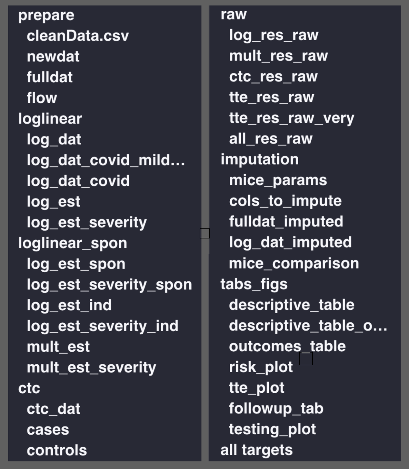
In big projects, I comment my _targets.R file so that I can use the RStudio outline pane to navigate the pipeline (my buggy function)

Key {targets} functions

• use_targets() gets you started with a _targets.R script to fill in
• tar_make() runs the pipeline and saves the results in _targets/objects/
• tar_make_future() runs the pipeline in parallel¹
• tar_load() loads the results of a target into the global environment
  (e.g., tar_load(clean_data))
• tar_read() reads the results of a target into the global environment
  (e.g., dat <- tar_read(clean_data))
• tar_visnetwork() creates a network diagram of the pipeline
• tar_outdated() checks which targets need to be updated
• tar_prune() deletes targets that are no longer in _targets.R
• tar_destroy() deletes the .targets/ directory if you need to burn everything down and start again

1. Note: {targets} is moving to a new distributed computing strategy using {crew}

Advanced {targets}

“target factories”

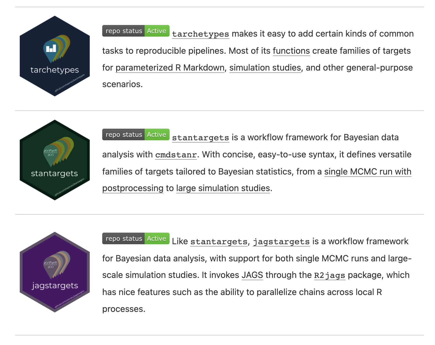
{tarchetypes}: reports

Render documents that depend on targets loaded with tar_load() or tar_read().

• tar_render() renders an R Markdown document
• tar_quarto() renders a Quarto document (or project)

Warning

It can’t detect dependencies like tar_load(ends_with("plot"))

What does report.qmd look like?

---
title: "My report"
---
```{r}
library(targets)
tar_load(results)
tar_load(plots)
```
There were `r results$n` observations with a mean age of `r results$mean_age`.
```{r}
library(ggplot2)
plots$age_plot
```

Because report.qmd depends on results and plots, it will only be re-rendered if either of those targets change.

Tip

The extra_files = argument can be used to force it to depend on additional non-target files

{tarchetypes}: branching

Using data from the National Longitudinal Survey of Youth,

_targets.R

library(targets)
library(tarchetypes)
tar_source()

targets_setup <- list(
  tar_target(
    csv,
    "data/nlsy.csv",
    format = "file"
  ),
  tar_target(
    dat,
    readr::read_csv(csv, 
      show_col_types = FALSE)
  )
)

R/functions.R

model_function <- function(outcome_var, 
                           sex_val, dat) {

  lm(as.formula(paste(outcome_var, 
      " ~ age_bir + income + factor(region)")) ,
     data = dat, 
     subset = sex == sex_val)
}

coef_function <- function(model) {
  coef(model)[["age_bir"]]
}

we want to investigate the relationship between age at first birth and hours of sleep on weekdays and weekends among moms and dads separately¹

1. Data and code at https://github.com/louisahsmith/targets-example

Option 1

Create (and name) a separate target for each combination of sleep variable ("sleep_wkdy", "sleep_wknd") and sex (male: 1, female: 2):

targets_1 <- list(
  tar_target(
    model_1,
    model_function(outcome_var = "sleep_wkdy", sex_val = 1, dat = dat)
  ),
  tar_target(
    coef_1,
    coef_function(model_1)
  )
)

… and so on…

tar_read(coef_1)

[1] 0.00734859

Option 2

Use tarchetypes::tar_map() to map over the combinations for you (static branching):

targets_2 <- tar_map(
  values = tidyr::crossing(
    outcome = c("sleep_wkdy", "sleep_wknd"),
    sex = 1:2
  ),
  tar_target(
    model_2,
    model_function(outcome_var = outcome, sex_val = sex, dat = dat)
  ),
  tar_target(
    coef_2,
    coef_function(model_2)
  )
)
tar_load(starts_with("coef_2"))
c(coef_2_sleep_wkdy_1, coef_2_sleep_wkdy_2, coef_2_sleep_wknd_1, coef_2_sleep_wknd_2)

[1] 0.00734859 0.01901772 0.02595109 0.01422970

Option 2, cont.

Use tarchetypes::tar_combine() to combine the results of a call to tar_map():

combined <- tar_combine(
  combined_coefs_2,
  targets_2[["coef_2"]],
  command = vctrs::vec_c(!!!.x),
)
tar_read(combined_coefs_2)

coef_2_sleep_wkdy_1 coef_2_sleep_wkdy_2 coef_2_sleep_wknd_1 coef_2_sleep_wknd_2 
         0.00734859          0.01901772          0.02595109          0.01422970 

command = vctrs::vec_c(!!!.x) is the default, but you can supply your own function to combine the results

Option 3

Use the pattern = argument of tar_target() (dynamic branching):

targets_3 <- list(
  tar_target(
    outcome_target,
    c("sleep_wkdy", "sleep_wknd")
  ),
  tar_target(
    sex_target,
    1:2
  ),
  tar_target(
    model_3,
    model_function(outcome_var = outcome_target, sex_val = sex_target, dat = dat),
    pattern = cross(outcome_target, sex_target)
  ),
  tar_target(
    coef_3,
    coef_function(model_3),
    pattern = map(model_3)
  )
)
tar_read(coef_3)

coef_3_85bbb1b6 coef_3_c47db1e2 coef_3_5ba8b6ec coef_3_19c76a86 
     0.00734859      0.01901772      0.02595109      0.01422970 

Branching

Dynamic	Static
Pipeline creates new targets at runtime.	All targets defined in advance.
Cryptic target names.	Friendly target names.
Scales to hundreds of branches.	Does not scale as easily for tar_visnetwork() etc.
No metaprogramming required.	Familiarity with metaprogramming is helpful.

From https://books.ropensci.org/targets/dynamic.html#branching

Branching

• The book also has an example of using metaprogramming to map over different functions
  • i.e. fit multiple models with the same arguments
• Static and dynamic branching can be combined
  • e.g. tar_map(values = ..., tar_target(..., pattern = map(...)))
• Branching can lead to slowdowns in the pipeline (see book for suggestions)

{tarchetypes}: repetition

tar_rep() repeats a target multiple times with the same arguments

targets_4 <- list(
  tar_rep(
    bootstrap_coefs,
    dat |>
      dplyr::slice_sample(prop = 1, replace = TRUE) |>
      model_function(outcome_var = "sleep_wkdy", sex_val = 1, dat = _) |>
      coef_function(),
    batches = 10,
    reps = 10
  )
)

The pipeline gets split into batches x reps chunks, each with its own random seed

{tarchetypes}: mapping over iterations

sensitivity_scenarios <- tibble::tibble(
  error = c("small", "medium", "large"),
  mean = c(1, 2, 3),
  sd = c(0.5, 0.75, 1)
)

tar_map_rep() repeats a target multiple times with different arguments

targets_5 <- tar_map_rep(
  sensitivity_analysis,
  dat |> 
    dplyr::mutate(sleep_wkdy = sleep_wkdy + rnorm(nrow(dat), mean, sd)) |>
    model_function(outcome_var = "sleep_wkdy", sex_val = 1, dat = _) |>
    coef_function() |> 
    data.frame(coef = _),
  values = sensitivity_scenarios,
  batches = 10,
  reps = 10
)

{tarchetypes}: mapping over iterations

tar_read(sensitivity_analysis) |> head()

           coef error mean  sd tar_batch tar_rep    tar_seed tar_group
1  0.0061384611 small    1 0.5         1       1 -1018279263         2
2 -0.0005346553 small    1 0.5         1       2  -720048594         2
3  0.0073674844 small    1 0.5         1       3 -1478913096         2
4  0.0039254289 small    1 0.5         1       4 -1181272269         2
5  0.0108489430 small    1 0.5         1       5   135877686         2
6  0.0029473286 small    1 0.5         1       6  -564559689         2

Ideal for sensitivity analyses that require multiple iterations of the same pipeline with different parameters

tar_read(sensitivity_analysis) |>
  dplyr::group_by(error) |> 
  dplyr::summarize(q25 = quantile(coef, .25),
                   median = median(coef),
                   q75 = quantile(coef, .75))

   error         q25      median         q75
1  large 0.001427986 0.007318120 0.011399772
2 medium 0.004158480 0.007770285 0.011367160
3  small 0.004058926 0.006614599 0.009004322

The end

• {targets} is a great tool for managing complex workflows
• {tarchetypes} makes it even more powerful
• The user manual is a great resource for learning more
• Play around with some of the examples I showed

Thanks!